How we sped up random forest processing, getting the lay of the land

I work on the team at that is responsible for job ad selection model. These things:

This model predicts the likelihood that a user will click on a given job relative to all the other jobs. At any given time there are a bunch of jobs on the job board that the current visitor can see, so we calculate the expectation for each job, then we perform a weighted random selection over those values.

The problem we have is that the model needs to be updated from time to time to account for changing market conditions. Basically, new technologies come out all the time and which kinds of technologies are being used on Stack Overflow changes over time and which kinds of jobs are being listed changes all the time.

In this most recent round of updating the model, we decided to go outside of our typical process of using a and instead decided to try out numerous kinds of other models. At the end of the day, the best model based on our selection criteria turned out to be a . A random forest is basically a collection of decision trees that all combine to make a prediction.

You may have heard of decision trees because they are the brunt of one of the biggest jokes in all of AI.

image source:

But it turns out they are quite powerful after all, especially when you use a lot of them together, like a random forest. I tend to get a little upset when I see that meme because the interesting part isn't really how they make the predictions, it's in how they are constructed, which is legitimate ML.

Training a random forest can be quite expensive however, and we were not able to feed it all of our sample data. Instead it was decided to try a similar model, which we could feed with much more data in the same amount of time. This is trained in a totally different manner, i.e. using , however on the prediction side it turns out to be almost exactly the same as a random forest.

So we have a new model, we hope it's going to be good, now we need to run a test which means we need to get this thing into a API that can be called from our ad server.

Try the easiest thing first

One problem we have had here is that most of our models are trained in the and then we have to convert to those models to run in C# which is what we use for pretty much all production stuff here at Stack Overflow.

It has been on our radar for a long time to try to run R in production so we can avoid the step of transfering the model to a new system. There has been more than one major mistake on account of that transfer and it would also reduce our time to push out new models once we get them from our data scientist.

So we tried it. And then we were like, okay, let's see how fast it is.

image source:

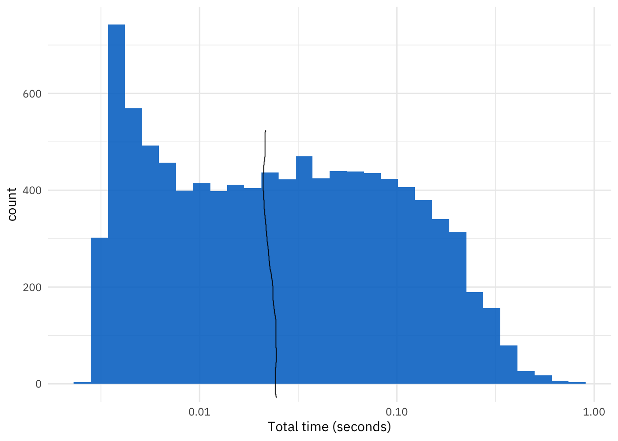
That's... ummm, not fast. That's about a 25 millisecond average time to score a single job. But wait, we have a lot of jobs on the job board at any time.

That's how many you can see right now if you live in the United States and you can see how many jobs are available in your area right now by visiting . And if we multiply that with the time it takes to score one job on average, we're looking at 3810 * 25ms = 95,250ms. That's a lot of ms to render a job ad. Too many in fact. I guess we need to take a look at our overall requirements.

The requirements

First off, the number of jobs fluctuates from time to time due to various marketing and syndication efforts, as well as the general seasonal fluctuations. We need to build in some buffer here, so let's say this needs to work for 5,000 jobs, and of course the more the merrier.

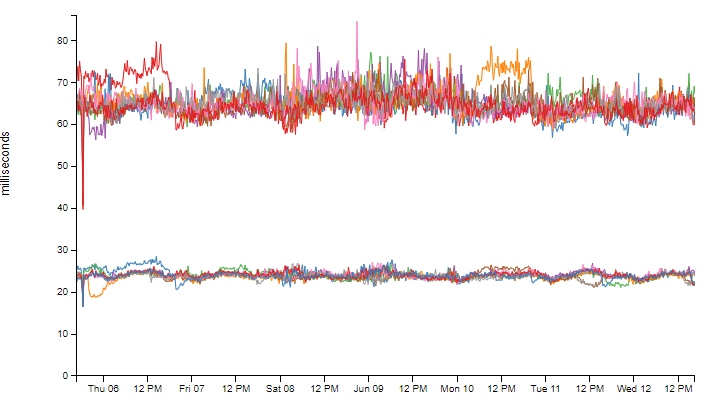
Looking at our current ad request times, it looks like the entire job selection process takes about 25 ms on average and roughly 65-70 ms for the 99th percentile. That's to do all the scoring and choosing of the jobs based on those scores. I'm not entirely sure how much of that time is the job selection process, but we should give ourselves some buffer here and let's just call it 25 ms to match what we have and we need to keep the 99th percentile under 65 ms.

This application runs on our web tier, the exact same boxes that Stack Overflow and all the other Stack Exchange sites run on. These boxes are getting slammed like crazy with requests. On our web tier, pretty much anything in the path of a request needs to be handled in a single-threaded manner. In order to test out something that operates in parallel would be a test all of it's own and is beyond the scope of this project.

We also need to be aware of the memory usage for this application. The request handling needs to allocate as little memory as possible but there is some leeway here because the boxes themselves run at about 80% memory capacity already. There are 64 GB of RAM on each of these boxes, and we need to keep some buffer in there, so going to the architecture team to ask for more than a couple gigabytes on each of these boxes is a pretty big ask. Whatever memory it takes to run a single request, we really need to multiply it times 48 because there are 48 cores on the box. If we want to stay under say 3 GB, then we have at most 62.5 MB per request.

And lastly, we really only care about making this specific model fast enough to run the test. It is not necessary to build a general purpose random forest implementation here, just something that can test the model we were given so we can verify if it is an improvement over our old model or not. It is totally fine to make concessions as necessary to support only this one instance, and if this model turns out to be better than what we currently have, then we might consider generalizing it to support a wider range of model instances.

So in short, the requirements for handling a single request are:

• must score 5,000 jobs for a user
• must complete in roughly 25 ms, and 99% of requests need to finish in under 65 ms
• must be single-threaded
• must use less than roughly 65 MB total
• all tricks are allowed as long as this one model instance works correctly

Let's stick to our bread and butter

We're much better at C# here than we are at R for performance critical applications. Additionally the most important thing to do right now is to verify that this new model is an improvement over the old model so building out a pipeline that included R in production was probably a lot of additional work we didn't need to consider doing for this anyway.

So we decided to write this in C# and we went with the most naive possible solution. Pretty much all the code to run the XGBoost model looks like this:

1
2
3
4
5
6
7
8
9
10
11
12
13
14
15
16
17
18
19
20
21
22
23
24
25
26
27
28
29
30
31
32
33
34
35
36
37
38
39
40
41
42
43
44
45
46
47
48
49
50
51
52
53

public sealed class DecisionTree
{
    public class DecisionTreeNode
    {
        public int FeatureIndex { get; set; }
        public double Value { get; set; }
        public int TrueBranch { get; set; }
        public int FalseBranch { get; set; }
    }

    const int LeafIndex = -1;

    private readonly DecisionTreeNode[] nodes;

    public DecisionTree(DecisionTreeNode[] tree)
    {
        nodes = tree;
    }

    public double Evaluate(double[] features)
    {
        var node = nodes[0];
        while(node.FeatureIndex != LeafIndex)
        {
            int nodeIndex = features[node.FeatureIndex] < node.Value ? node.TrueBranch : node.FalseBranch;
            node = nodes[nodeIndex];
        }
        return node.Value;
    }
}

public sealed class RandomForest
{
    private readonly DecisionTree[] trees;

    public RandomForest(DecisionTree[] trees)
    {
        this.trees = trees;
    }

    public double EvaluateProbability(double[] instance)
    {
        var sum = trees.Sum(t => t.Evaluate(instance));
        var result = Logit(sum);
        return result;
    }

    // this converts the output to a probability
    private double Logit(double value)
    {
        return 1f / (1f + Math.Exp(-value));
    }
}

That's basically all the work part of it. I left off the parsing code because it's not particularly important but so you are aware of what the actual output from the XGBoost model in R looks like, here's a snippet:

booster[0]
0:[f0<0.99992311] yes=1,no=2,missing=1,gain=97812.25,cover=218986
1:leaf=-0.199992761,cover=27584.75
2:[f17<0.000367681001] yes=3,no=4,missing=3,gain=10373.0732,cover=191401.25
3:[f2<0.5] yes=5,no=6,missing=5,gain=4121.85938,cover=103511.5
5:[f6<0.00216802233] yes=9,no=10,missing=9,gain=873.340759,cover=50533.25
9:[f732<0.5] yes=17,no=18,missing=17,gain=515.368896,cover=33356.75
17:leaf=-0.00213295687,cover=25503.5
18:leaf=-0.0314288437,cover=7853.25
10:[f732<0.5] yes=19,no=20,missing=19,gain=276.522034,cover=17176.5
19:leaf=0.0253729131,cover=13474
20:leaf=-0.00548130181,cover=3702.5
6:[f734<0.237819463] yes=11,no=12,missing=11,gain=2141.23145,cover=52978.25
11:[f8<0.00104575348] yes=21,no=22,missing=21,gain=566.334961,cover=35689
21:leaf=-0.0620479584,cover=24457.5
22:leaf=-0.0349165387,cover=11231.5
12:[f762<0.308019817] yes=23,no=24,missing=23,gain=483.886719,cover=17289.25
23:leaf=-0.0144120604,cover=16450.5
24:leaf=0.063411735,cover=838.75
4:[f2<0.5] yes=7,no=8,missing=7,gain=2694.23291,cover=87889.75
7:[f27<0.000739371637] yes=13,no=14,missing=13,gain=928.447266,cover=44100.5
13:[f732<0.5] yes=25,no=26,missing=25,gain=285.069702,cover=17082.25
25:leaf=0.032621529,cover=13427.25
26:leaf=0.00112144416,cover=3655
14:[f285<0.000919258455] yes=27,no=28,missing=27,gain=421.745117,cover=27018.25
27:leaf=0.0483669229,cover=20145
28:leaf=0.077062957,cover=6873.25
8:[f734<0.103942066] yes=15,no=16,missing=15,gain=1591.2124,cover=43789.25
15:[f101<0.000240761583] yes=29,no=30,missing=29,gain=608.92157,cover=24192.75
29:leaf=-0.0209285971,cover=14574.75
30:leaf=0.0114876805,cover=9618
16:[f722<0.5] yes=31,no=32,missing=31,gain=601.422363,cover=19596.5
31:leaf=0.0258833747,cover=18429.75
32:leaf=0.099892959,cover=1166.75
booster[1]
0:[f0<0.99992311] yes=1,no=2,missing=1,gain=80168.1719,cover=218645.734
1:leaf=-0.181867003,cover=27310.75
2:[f17<0.000390548841] yes=3,no=4,missing=3,gain=8405.98535,cover=191334.984
3:[f2<0.5] yes=5,no=6,missing=5,gain=3338.54272,cover=103498.18
5:[f5<0.000531250262] yes=9,no=10,missing=9,gain=750.746765,cover=50538.3281
9:[f732<0.5] yes=17,no=18,missing=17,gain=355.950684,cover=32388.959
17:leaf=-0.00289925188,cover=24663.1035
18:leaf=-0.0274959896,cover=7725.85449
10:[f732<0.5] yes=19,no=20,missing=19,gain=279.289886,cover=18149.3711
19:leaf=0.0230532587,cover=14319.1934
20:leaf=-0.00734602008,cover=3830.17749
6:[f734<0.237819463] yes=11,no=12,missing=11,gain=1736.53467,cover=52959.8516
11:[f5<0.000720986514] yes=21,no=22,missing=21,gain=514.774414,cover=35668.0508
21:leaf=-0.0571310222,cover=22939.1699
22:leaf=-0.0320498347,cover=12728.8799
12:[f722<0.5] yes=23,no=24,missing=23,gain=468.159485,cover=17291.8027
23:leaf=-0.0137320729,cover=16250.6074
24:leaf=0.0554070361,cover=1041.19482
4:[f2<0.5] yes=7,no=8,missing=7,gain=2186.99561,cover=87836.8047
7:[f27<0.000739371637] yes=13,no=14,missing=13,gain=755.193359,cover=44065.7109
13:[f668<0.5] yes=25,no=26,missing=25,gain=245.545715,cover=17078.1777
25:leaf=0.0203356724,cover=16096.4053
26:leaf=0.0718296021,cover=981.772095
14:[f58<0.000670915877] yes=27,no=28,missing=27,gain=312.375,cover=26987.5352
27:leaf=0.0368296206,cover=10639.0859
28:leaf=0.0588531196,cover=16348.4482
8:[f734<0.237819463] yes=15,no=16,missing=15,gain=1328.46338,cover=43771.0977
15:[f27<0.000467836275] yes=29,no=30,missing=29,gain=631.899902,cover=28666.8477
29:leaf=-0.0222451035,cover=11761.168
30:leaf=0.00793752726,cover=16905.6797
16:[f722<0.5] yes=31,no=32,missing=31,gain=362.48999,cover=15104.248
31:leaf=0.0279367212,cover=14043.1475
32:leaf=0.0885346606,cover=1061.10071

This snippet shows two trees, delimited by the lines that start with booster[ and there are 1,000 of these trees. Due to the way this model was trained, the missing branch, which you would normally take when a feature is missing from the sample, is always the "no" branch. This is because we replace all values with 0 if they are missing, and all features have a positive value in our problem space. The gain and cover variables are just output from the model for your information but do not affect the tree at all. The first number is the index of the line that is referred to by the "yes" and "no" parameters. The features are numbered 0 through about 840 in our data, so when you see fXXX it means feature number XXX in the input. The input to these, as you can see from the Evaluate function is just an array of doubles.

How close are we?

Let's try it out real fast, and see. This is just using a simple timer wrapped around running this code with 5000 examples. One caveat here, make sure you run this in release mode or your times will be wildly different.

[6/20/19 4:02:34 AM] Time taken for 5000 evaluations: 319.5548 ms

Hey that's not so bad, only a factor of about 12-13 to go. I should point out here that when you're trying to reach a specific performance goal, the actual machine you're going to be running this on makes a difference. My dev box gets an update about every other year, and is much more powerful than a lot of our production servers, especially the ones this will be running on. In fact if you run this on processors released in the last year or two, you might see times as low as 220 ms, like I did on my laptop which only 4 months old. [obligatory works-on-my-machine badge here] In an ideal world, we would run this test on the machine we care about, but since we're so far from meeting our requirements already, it's not time for that yet.

But wait up, let's not get ahead of ourselves, let's verify this is actually generating the correct values too. Keep in mind that there are a bunch of samples here that we used for the timing that we can now use to verify it is spitting out the correct values. These samples, and the expected outputs, were provided to us by our data scientist.

1
2
3
4
5
6
7
8
9
10
11

RandomForest model; // loaded in test setup
double[][] samples; // loaded in test setup
const int probablity_feature_index = 840;

foreach(var sample in samples)
{
    var actual = model.EvaluateProbability(sample);
    var expected = sample[probablity_feature_index];
    Assert.InRange(actual, expected - 1e-06, expected + 1e-06);
}
output.WriteLine("Correctness verified.");

[6/20/19 4:02:34 AM] Correctness verified.

So \o/ we're on the right track!

Let's also take a second to realize that the biggest win we're going to see here at all is that moving away from the tooling we are not familiar with, i.e. the R API described above, to something we are much better with. We were able to reduce the time for a single sample evaluation from roughly 25 ms to roughly 0.047 ms which is roughly three orders of magnitutude. I want to be clear, this is not because R is slow, it's because we are not familiar enough with R to write efficient code. The rest of this entire series is about grinding out as much of that last order of magnitude as possible.

What's next?

Next time we're going to take a look at some really basic improvements which will net us a fair amount of win. The first step for designing anything is to get it working correctly and set a baseline for performance. These next few things we address will be very common tips that can show some major improvements in your applications with only minor changes.

If you are interested in following along and trying this stuff out for yourself, please clone and run the naive tests as shown in the readme.

How we sped up random forest process series

• Getting the lay of the land
• Lots of common performance patterns